Introduction To Machine Learning With Python
Of course, everybody now is talking about machine learning and how robots will take over life! Lots of movies talked about how artificial intelligence will advance and affect our lives for better or worse. This got all people thinking, is that really what’s going to happen? How does machine learning work?
Well, that’s not what we’re here to answer! (unfortunately)
We’re here to give you (the one who is interested in machine learning and data science) a hands-on experience on how to develop machine learning and use it to solve real (and important) life problems. Yes, we will give you some basic concepts and theories in machine learning and its related fields but will not dig deep into them.
In normal coding, you tell the computer exactly what to do, and then they do it very precisely. But there are lots of situations or problems that this won’t be an option. It might be that the problem is too complex that you can’t write a specific set of rules or instructions to give. Also, it might be that the process of you giving the time and effort to define and set these rules is not worth it, or you don’t have much time and need a fast answer. The diversity and complexity of the problems make it truly hard if you don’t seek help in some other way.
This is where machine learning comes in.
Machine learning is the science of making the computer (a machine) learn from data and act on its own upon this experience. As you can see, the core of this process is the data itself, and the machine learns from it on its own (no specific coding involved). To make a machine learn, we have 3 important parts to consider; data, algorithm, and model.
Simply, the model uses the algorithm (which is the technique on how to learn from data) to learn from the data. After this learning process, your model is well trained and can predict other new data entries. It might seem straightforward forward but it’s truly not. Picking the right algorithm to use is a challenge, and filtering the data to be ready for the model to learn on is a challenge. Boosting the model’s accuracy is a challenge.
Let’s take an example of how this works. Say you need the computer to identify you by face recognition using a camera. Could you identify the set of rules to tell the computer how to do so? Most likely not. Even if you do, it’ll be a headache trying and you’ll take tremendous time. So, normal coding is not an option.
So, you go with a machine learning approach. You get 50 images of yourself including your face (the data), and you create a model with some algorithm that breaks images down and gets important features out of them (feature engineering), and using some algorithm it trains on these numbers and comes up with the set of rules itself so it can identify your face.
Now you can use this model for your purpose. It can now do the task as it learned on its own.
Now let’s talk about the process that you (a developer) take to create a machine learning model.
1. You first set up your data
Which includes reading the data, cleaning it (e.g. removing noise values, adding some missing values, etc.), and getting the important features out of it.
2. Next, choosing the right algorithm
There are lots of algorithms out there, you need to choose the right one based on the input data and the output you want. Some of them are quick in learning but slow in predicting, some are the opposite. According to your situation, you’ll identify what you need.
3. Then, Creating and “teaching” the model
Here, you give your data to a model that uses the algorithm you chose and start learning from it until finished.
4. After that you test your model
You now test the model by providing new data that it didn’t know about and measuring its accuracy and efficiency. If it’s good, congrats! you’re done and now can use it. But it might need changes, more data modifications, another algorithm, another set of data, etc. In this case, you’ll kind of repeat the process above until you’re done.
5. Finally, Use the model
Once you’re done, you can now use the model you’ve created in predicting and solving the problem you needed.
Machine Learning With Python: Getting started
Machine Learning has a lot more than we talked about, but we think that’s enough talking, let’s start doing it! And you will understand more while practicing and seeing the process in front of you step by step.
But first, let’s talk about Python for a little bit. Python is a great language when dealing with machine learning, it has so many useful packages that we can use to create our machine learning model. Let’s see some of these packages in action
NumPy
Numpy is the fundamental package for scientific computing with Python. It has tons of functionalities in statistics and maths.
Make sure you have it on your machine using pip pip install numpy or conda conda install numpy.
# Let us import numpy and play a little with it
import NumPy as np # np is the famous alias for NumPyNP Arrays
# The most powerful point in NumPy is its array
# np.array has attributes and properties that will make you love it
# Let's check them.
# this is how we create them from a regular python list
a = np.array([1, 2, 3, 4, 5, 6])
a
# for simplicity we call them 'ndarrays'
# short for number of dimensions
# since we can make them in any number of dimensions
# We can print the array's number of dimensions by:
a.ndim
# a 1 D-array as expected# And to find its shape we can write
a.shape
# 6 elements on a 1 dimensional array
# No surprises until now# Another powerful feature for numpy arrays is that
# we can change the shape of an existing array
# for example a 1 dimensional array forming it to 2 dimensions
# and vice versa
# np.arrays has a function called reshape for this process
# the function 'numpy.array.reshape()' takes the new shape of
# the array as a tuple (rows_number, columns_number)
# and returns a new copy of the array with new shape
b = a.reshape((3,2))
b# Now if we check the shape of b
# it won't be (6,)- 6 elements in a 1-D array
b.shape
# (3, 2) means 3 rows and 2 columns # Now, what if we wanted to change a value in b
# as this
b[0][0] = 15
b
# what do you think will happen to a?a
# Oh! The change in b were applied here too!
# Note!
# numpy is very efficient. It eliminates processes whenever possible
# that's why b is not an independent copy from a
# it's just a new view# But if you want an independent true copy;
# we will use the function 'numpy.array.copy()'
c = a.reshape((3,2)).copy()# Now, if we tried to change a it won't affect c
# and vice versa
c[1][0] = 50
c# Let us remove the doubts and print a again
a
# now the value 3 is still here.# An important property for ndarrays
# is operations propagation it means
# Simple operations can be applied over
# all the elements one by one
# and it's super fast
a*2
# this multiplied all the elements by 2# raise each element to the power 2
a**2
# Interesting, right?# Remember? we couldn't do that in the regular python lists
li = [15, 2, 3, 4, 5, 6]
li**2Indexing
# Another unique functionality is its way of accessing elements
# We can use another nd.array as list of indexes for the original array

# it will return from the element at index 2 to the element at index 4
a[np.array([2, 3, 4])]
# Of course this works too.
a[1:3]# and this
a[0]# Back to the operation propagation
# we can do the same with relational operations
a < 5# it allowed us to filter the list based on this condition
a[a < 5]# we can even go further and make values change based on the filter
a[a < 5] = 0
anp.NaN
# while gathering data we may miss some values
# or get them in a wrong form
# for this case we have numpy's value NAN
# short for not a number
# if at any data point numpy didn't find
# the desired value it will keep it as a nan value
c = np.array([1, 2, np.NAN, 3, 4])
c
# check nan values in an array
np.isnan(c)# filter them out
c[~np.isnan(c)]Run Time Comparison: Python Native Lists VS NumPy
# we kept talking about its speed and efficiency
# but is it really true?
# I will let you see yourself
# let's see how it performs against python lists

import timeit
python_native_time = timeit.timeit('sum(x**2 for x in range(1000))', number=10000)

np_time = timeit.timeit('na.dot(na)',
                        setup="import numpy as np; na=np.arange(1000)",
                        number=10000
                       )

print("Normal Python: {} sec".format(python_native_time))
print("NumPy: {} sec".format(np_time))

# 6 times faster!
# Cool!
Data Types
Unfortunately, for the sake of speed, we made some sacrifices. nd.arrays don’t have the types of flexibility that lists have.
a = np.array([1,2,3])
a.dtype
np.array([1, "text", set([1,2,3])])Scipy and Matplotlib
Scipy is a package containing fundamental algorithms for scientific computing in Python. It’s a fantastic tool along with Numpy (as it is built on top of it) and is a great building block for machine learning packages and algorithms.
Scipy has lots of useful sub packages like IO, stats, optimize, and others.
Matplotlib is a python library for visualization and plotting data into a figure. It’s very handy and helps you see the data and watch how they change or interact. It is used along with NumPy and scipy to provide you with the full experience you require.
Make sure you have them on your machine using pip pip install scipy matplotlib or conda conda install scipy matplotlib.
We won’t talk much here about scipy and matplotlib but let’s have a quick example.
# let's first import all packages
import matplotlib.pyplot as plt # importing the pyplot subpackage
from scipy import interpolate  # importing the interpolate subpackage
import numpy as np

# let's get first an array to be our x axis
# with values from an interval using np.arange()
x = np.arange(5, 20)
x
# let's then get an array to be our y axis
# with exponential values from the x list we've just generated
y = np.exp(x/3.0)
y# let's now use the interpolate subpackage
# to interpolate other values according to our 2 arrays
# the interp1d() returns a function whose call method
# uses interpolation to find the value of new points
# according to the given Xs and Ys
f = interpolate.interp1d(x, y)
f(10.5)# now, let's use it to
x1 = np.arange(6, 12, step=0.5)
y1 = f(x1) # use interpolation function returned by `interp1d`
[x1[:5], y1[:5]]# let's now plot them using the plot
plt.plot(x, y, x1, y1) # draw into a figure the 2 lines
plt.show() # show the figure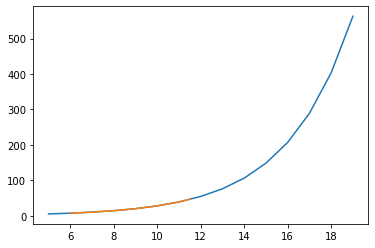
Now, you have a good idea about how to use NumPy, scipy, and matplotlib.
Enough with the theory and let’s play with the code.